Lissajous curve

The animation below shows the curve adaptation with continuously increasing fraction from 0 to 1 in steps of 0.01. (δ=0)

Below are examples of Lissajous figures with δ = π/2, an odd natural number a, an even natural number b, and |a − b| = 1.

• 

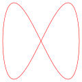  a = 2, b = 1 (2:1)
• 

  a = 3, b = 2 (3:2)
• 

  a = 3, b = 4 (3:4)
• 

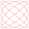  a = 5, b = 4 (5:4)

Generation

Prior to modern electronic equipment, Lissajous curves could be generated mechanically by means of a harmonograph.

Practical application

Lissajous curves can also be generated using an oscilloscope(as illustrated). An octopus circuit can be used to demonstrate the waveform images on an oscilloscope. Two phase-shifted sinusoid inputs are applied to the oscilloscope in X-Y mode and the phase relationship between the signals is presented as a Lissajous figure.
On an oscilloscope, we suppose x is CH1 and y is CH2, A is amplitude of CH1 and B is amplitude of CH2, a is frequency of CH1 and b is frequency of CH2, so a/b is a ratio of frequency of two channels, finally, δ is the phase shift of CH1.
A purely mechanical application of a Lissajous curve with a=1, b=2 is in the driving mechanism of the Mars Light type of oscillating beam lamps popular with railroads in the mid-1900s. The beam in some versions traces out a lopsided figure-8 pattern with the "8" lying on its side.

Application for the case of a = b

In this figure both input frequencies are identical, but the phase variance between them creates the shape of an ellipse.

Top: Input signal as a function of time, Middle: Output signal as a function of time. Bottom: resulting Lissajous curve when output is plotted as a function of the input. In this particular example, because the output is 90 degrees out of phase from the input, the Lissajous curve is a circle.

When the input to an LTI system is sinusoidal, the output is sinusoidal with the same frequency, but it may have a different amplitude and some phase shift. Using an oscilloscope that can plot one signal against another (as opposed to one signal against time) to plot the output of an LTI system against the input to the LTI system produces an ellipse that is a Lissajous figure for the special case of a = b. The aspect ratio of the resulting ellipse is a function of the phase shift between the input and output, with an aspect ratio of 1 (perfect circle) corresponding to a phase shift of and an aspect ratio of (a line) corresponding to a phase shift of 0 or 180 degrees. The figure below summarizes how the Lissajous figure changes over different phase shifts. The phase shifts are all negative so that delay semantics can be used with a causal LTI system (note that −270 degrees is equivalent to +90 degrees). The arrows show the direction of rotation of the Lissajous figure.

A pure phase shift affects the eccentricity of the Lissajous oval. Analysis of the oval allows phase shift from an LTI system to be measured.